Why Neural Networks Learn: Loss Functions and the Taylor Approximation

September 26, 2026 11 min read

There is a sentence, repeated in every introduction to machine learning, that everyone nods at and almost no one stops to interrogate: the network learns by minimizing the loss. It sounds like an explanation. It is actually a riddle wearing an explanation's clothes. What does it mean for a pile of numbers to "learn"? What is "loss," that minimizing it should produce intelligence? And by what mechanism does anything with millions of moving parts find its way to the bottom of anything?

This post takes the sentence apart and rebuilds it from first principles—with the math derived, not quoted, and the code written out, not hand-waved. The machinery underneath is older than the computer, older than statistics as a discipline, and—this is the part worth sitting with—almost embarrassingly simple once you see it.

Learning is search

Begin with the least mysterious object in the story: a function. A neural network, stripped of metaphor, is a function f(x; w). It takes an input x—pixels, words, a row of lab measurements—and produces an output. The w is a long list of numbers, the weights, which determine which function it is. Change the weights, change the behavior.

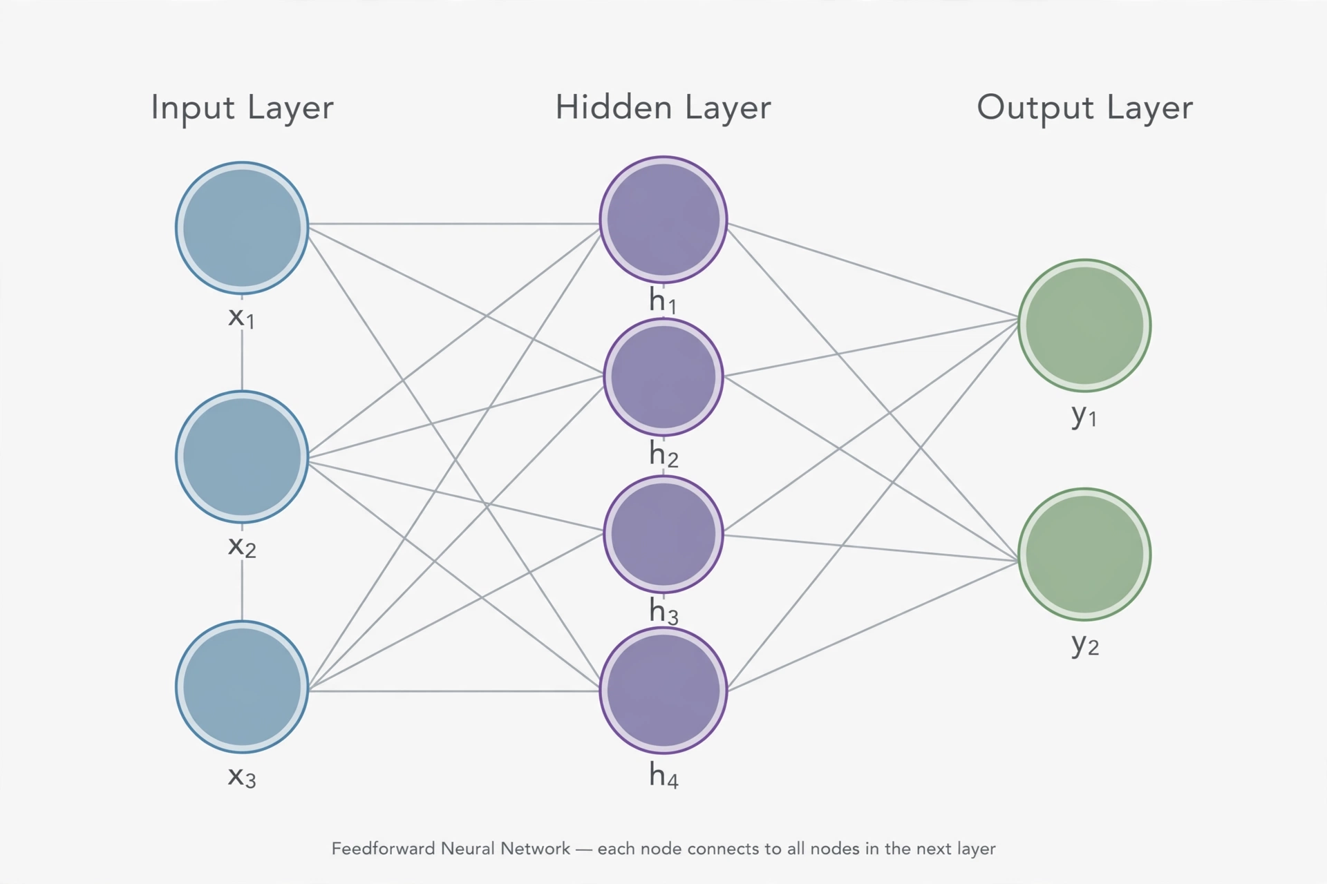
A small feedforward neural network: functions nested inside functions

"Learning" is the claim that we can find weights that make the function's outputs match reality on examples we show it. That is all it is. Not understanding, not insight—search. Somewhere in the vast space of possible weight settings sits one (many, actually) that classifies the images correctly, and learning is the process of walking toward it.

The moment you accept this framing, the mystical problem becomes a practical one, and it splits cleanly in two. First: how do you measure how wrong the current weights are? Second: given that measurement, how do you find better weights? The answers are the loss function and the optimizer, and both are deeper than they look.

Wrongness, made measurable

You cannot minimize what you cannot score. So the first invention is a number that says how bad the current predictions are: the loss.

The most famous one is the squared error. For each example, take the difference between prediction and truth, and square it. Why square? The textbook answer—differentiability, penalizing large errors more than small ones—is true but shallow. The deep answer is that the squared error smuggles in an assumption about the world: it is what you get if you assume the truth equals your prediction plus Gaussian noise, and then ask which weights make the observed data most likely. Squaring is maximum likelihood wearing a costume. Every time you minimize mean squared error, you are quietly doing statistics from 1809—Gauss's least squares, famously used to relocate the lost asteroid Ceres, now grading homework for image classifiers.

Classification gets its own loss, cross-entropy, and it deserves its derivation too. Suppose the model doesn't output an answer but a probability over answers. How surprised should we be when the true answer arrives? If the model gave it probability p, define surprise as −log p: certain predictions that come true carry no surprise; confident wrong predictions carry enormous surprise. The loss is the average surprise. Minimizing it is, again, maximum likelihood—choose the weights that make the training data least surprising. Same principle as squared error, one level up the ladder of abstraction.

Here is the pattern to pocket: every loss function is an assumption about the world, written as arithmetic. Choose squared error and you assume Gaussian noise. Choose cross-entropy and you assume the data was generated by the probabilities you output. The loss is not a law of nature; it is a bet. Deep learning works as well as it does partly because these particular bets are usually good ones.

The math of wrongness

Now let's stop describing the loss and differentiate it, because the derivative is where the learning lives.

Mean squared error over n examples:

L(w) = \frac{1}{n}\sum_{i=1}^{n}\big(f(x_i; w) - y_i\big)^2

Differentiate with respect to one weight $w_j$ (chain rule—it will be back shortly):

\frac{\partial L}{\partial w_j} = \frac{2}{n}\sum_{i=1}^{n}\underbrace{\big(f(x_i; w) - y_i\big)}_{\text{how wrong}} \cdot \underbrace{\frac{\partial f}{\partial w_j}}_{\text{how much this knob mattered}}

Read it in words: the gradient is the error signal times the local sensitivity, averaged over examples. Hold onto that shape—every gradient in deep learning looks like this: how wrong you were, multiplied by how much this particular weight contributed. Backpropagation, when we reach it, is just an efficient way to compute the second factor for every weight at once.

Cross-entropy has an even prettier derivative. With logits $z_j$, softmax probabilities $p_j = e^{z_j}/\sum_k e^{z_k}$, and one-hot truth $y$:

L = -\sum_j y_j \log p_j \quad\Longrightarrow\quad \frac{\partial L}{\partial z_j} = p_j - y_j

Prediction minus truth. After all the exponentials and logarithms, the gradient of the most widely used classifier loss in existence simplifies to how wrong the probabilities were. When the math collapses this cleanly, it is usually telling you the formulation was the right one.

The hard part

Now the genuinely difficult half. The loss is a function of the weights—millions of them. Somewhere in that million-dimensional space is a valley floor. How do you find it?

Brute force is hopeless. Visualization is hopeless too—and readers of this blog's earlier post on thinking in many dimensions will recognize the required move: stop trying to see the landscape, and compute with it instead. What we need is a local question with a local answer: standing here, at these weights, which way is down?

The answer is three hundred years old.

Taylor's microscope

In 1715, Brook Taylor published the observation that near any point, a complicated curve looks simple. Zoom in close enough on any smooth function and it becomes a straight line; pull back slightly and it becomes a parabola. Formally:

f(a + h) \approx f(a) + f'(a)\cdot h + \tfrac{1}{2}f''(a)\cdot h^2

Where does this come from? Demand that the approximation match the function's value at $a$ (first term), its slope at $a$ (second term), and its curvature at $a$ (third term). Each term fixes one more derivative, and the polynomial that matches all three hugs the curve near $a$—the tangent line briefly, the parabola longer.

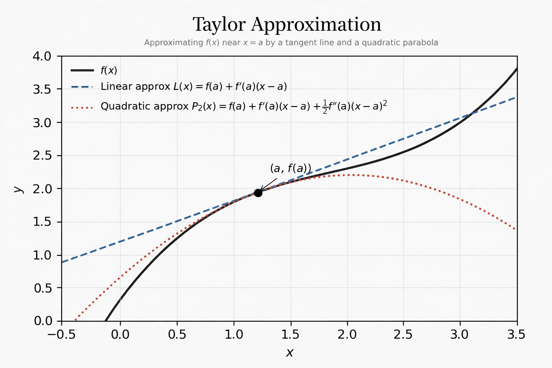
Taylor approximation: a curve, its tangent line, and the closer-hugging parabola

Dwell on what this buys. You do not need the whole landscape. You do not need to see the valley. You need only the ground under your feet—the value, the slope, the curvature right here—and Taylor hands you a simple, solvable model of the neighborhood. The unknown becomes the approximately known, locally, and locally is enough if you are willing to re-ask the question after every step.

Walking downhill with a local map

Gradient descent is Taylor approximation, iterated. The first-order Taylor model says the loss decreases fastest in the direction opposite the gradient—the direction of steepest descent. So: compute the slope, take a small step downhill, and repeat. That is the entire algorithm. Augustin-Louis Cauchy wrote it down in 1847, a century and a half before anyone had a use for it at scale.

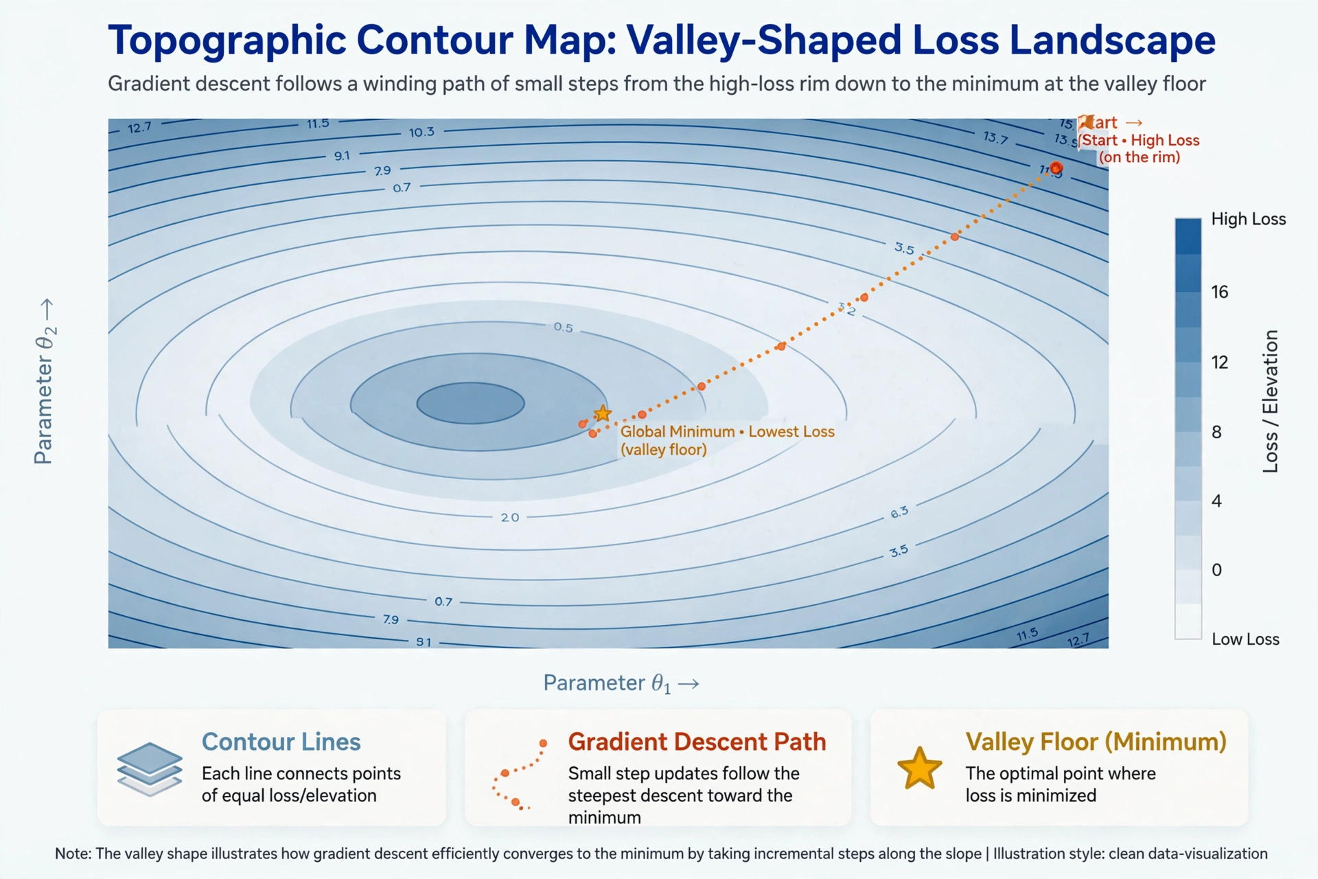
Gradient descent: small steps winding down a loss landscape to the minimum

Everything fiddly about training neural networks lives in one word of that description: small. The step size—the learning rate—is the whole game, because Taylor's map is only trustworthy nearby. Step too far and the linear approximation lies to you: you overshoot the valley and climb the far wall, or diverge entirely. Step too timidly and you crawl. Every learning-rate schedule, every warmup and decay, is an attempt to keep steps inside the radius where the local map is honest.

The failure modes are Taylor's failure modes, and naming them this way demystifies half of optimization folklore. Ravines: the landscape curves sharply in one direction and gently in another; the linear model is locally correct but globally naive, so you zigzag across the ravine instead of gliding down it. Saddle points: the gradient is near zero, so first-order Taylor reports "flat"—but flat can be a mountain pass, not a valley floor, and pure gradient descent lingers there, confused. Local minima: the map is honest and you have arrived—at the bottom of the wrong valley.

And then the miracle, which deserves a pause: this naive procedure—ask which way is down, step, repeat—trains models with billions of parameters. It should not work as well as it does. That it does is one of the great empirical facts of our century, and nobody fully understands why the valleys it finds generalize so well. The algorithm is 1847; the mystery is current.

Code: the optimizer in fifteen lines

Everything above fits in a few lines of NumPy. Minimize $f(x) = x^2$—we know the answer is $x = 0$; the point is the procedure, which never uses that knowledge:

import numpy as np

def f(x):    return x**2   # the "loss landscape"
def grad(x): return 2*x    # its slope — the gradient

x = 8.0    # start far from the answer
lr = 0.1   # step size: how far we trust the local map
for step in range(50):
    x = x - lr * grad(x)   # first-order Taylor, iterated
    print(f"step {step:2d}  x={x:+.3f}  loss={f(x):.3f}")

The loss falls: 64 → 41 → 26 → … → 0. That loop—evaluate, differentiate, step—is the entire optimizer. Every training run in history is this loop with a fancier grad().

The parabola you can't afford

First-order Taylor gives gradient descent. Second-order Taylor gives Newton's method: instead of stepping downhill, jump straight to the bottom of the local parabola. One step, done—when the parabola is accurate.

Why isn't everything Newton's method? Because curvature in n dimensions is an n×n matrix, the Hessian, and for a billion parameters that matrix has a quintillion entries. You cannot store it, let alone invert it. The parabola is the better map and you cannot afford to draw it.

So the field cheats, cleverly. Momentum remembers past gradients, letting the optimizer barrel through ravines instead of zigzagging—a poor man's curvature, bought with memory instead of matrices. Adam and its cousins adapt the step size per parameter, effectively preconditioning the landscape with a cheap diagonal guess at curvature. Every modern optimizer is Taylor's second order, approximated on a budget. The through-line of 150 years of optimization research: the full Taylor expansion is the truth; everything practical is a negotiation with its cost.

The chain rule, industrialized

One loose end remains, and it is the one that makes the whole scheme computable. The gradient of a million-parameter function sounds like a million separate hard problems—until you notice the network's structure. A neural network is functions nested inside functions, layer after layer, and the derivative of a composition is the chain rule:

\frac{dz}{dx} = \frac{dz}{dy}\cdot\frac{dy}{dx}

Backpropagation is the chain rule, applied systematically, with bookkeeping. The forward pass computes values flowing left to right; the backward pass computes, for every weight, how much it mattered—the derivative of the loss with respect to that weight—flowing right to left, reusing each layer's work instead of recomputing it. What would naively cost O(n²) drops to O(n). Popularized by Rumelhart, Hinton, and Williams in 1986, it is the reason the gradient—the "which way is down" signal—can be obtained at all at scale.

If gradient descent is the walking, backpropagation is the compass. One line of intuition covers it: credit assignment, done with calculus.

Code: a neural network from scratch

Here is the whole post so far, running. A tiny 1→16→1 network learns $y = \sin(x)$—forward pass, MSE loss, hand-derived backprop, gradient descent:

import numpy as np

# Toy data: learn y = sin(x)
xs = np.linspace(-np.pi, np.pi, 200).reshape(-1, 1)
ys = np.sin(xs)

rng = np.random.default_rng(0)
W1 = rng.normal(0, 1, (1, 16)); b1 = np.zeros((1, 16))
W2 = rng.normal(0, 1, (16, 1)); b2 = np.zeros((1, 1))

def forward(x):
    h = np.tanh(x @ W1 + b1)
    return h @ W2 + b2, h

lr = 0.05
for epoch in range(2000):
    pred, h = forward(xs)
    err = pred - ys
    loss = np.mean(err**2)

    # Backprop: the chain rule, right to left.
    dloss = 2 * err / len(xs)            # d(mean(err^2)) / d(pred)
    dW2 = h.T @ dloss                    # how much W2 mattered
    db2 = dloss.sum(axis=0, keepdims=True)
    dh = (dloss @ W2.T) * (1 - h**2)     # ... through tanh ...
    dW1 = xs.T @ dh                      # ... to W1
    db1 = dh.sum(axis=0, keepdims=True)

    # Gradient descent: one small step downhill.
    W1 -= lr * dW1; b1 -= lr * db1
    W2 -= lr * dW2; b2 -= lr * db2

    if epoch % 500 == 0:
        print(f"epoch {epoch:4d}  loss={loss:.4f}")

Loss falls from ~0.5 to ~0.001. A random pile of numbers, shown 200 points of a sine wave, arranges itself into a sine-wave machine—by walking downhill, one Taylor-approved step at a time. Nothing in this program "understands" trigonometry. It is search, mechanized.

The real stuff

Now the reveal: this exact loop is what PyTorch runs. The forty lines above compress to this, line for line:

import torch

xs = torch.linspace(-torch.pi, torch.pi, 200).reshape(-1, 1)
ys = torch.sin(xs)

model = torch.nn.Sequential(
    torch.nn.Linear(1, 16), torch.nn.Tanh(), torch.nn.Linear(16, 1))
opt = torch.optim.Adam(model.parameters(), lr=0.05)

for epoch in range(2000):
    opt.zero_grad()
    loss = torch.nn.functional.mse_loss(model(xs), ys)
    loss.backward()   # backprop — the chain rule, automated
    opt.step()        # gradient descent — the walking, automated
    if epoch % 500 == 0:
        print(f"epoch {epoch:4d}  loss={loss.item():.4f}")

The mapping is exact: model(xs) is our forward(), mse_loss is our loss, backward() replaces every hand-derived dW line (autograd is backprop, applied to arbitrary code), and opt.step() replaces the manual W -= lr*dW (Adam just chooses smarter step sizes). The frameworks contain no new mathematics—they are the ideas of this post, industrialized: the chain rule done by software, the stepping done on GPUs, the loop run over billions of examples.

So what is "the real stuff," the part that turned these 19th-century ideas into the defining technology of our time? It is not a secret sixth idea. It is scale applied to these five: parameter counts from dozens to trillions, datasets from hundreds of points to the internet, and hardware that computes a million-dimensional gradient—that "which way is down" signal—in milliseconds. The sine-wave toy above and a frontier language model differ in degree, not in kind. You now understand, mechanically, what happens inside every training run on earth.

The stack, in one paragraph

Neural network: a flexible family of functions, parameterized by weights. Loss: wrongness made measurable—and every loss is a bet about the world, usually a maximum-likelihood bet in disguise. Taylor approximation: the local map, the ground under your feet made solvable. Gradient descent: walking downhill with that map, re-drawn at every step. Backpropagation: drawing the map efficiently, via the chain rule. Data: the territory the map must match.

Everything since 2012—the architectures, the scale, the emergent capabilities—is engineering on top of these five ideas. Four of them are pre-1900 mathematics. The fifth is the computer. The riddle from the opening dissolves: the numbers "learn" because wrongness is a landscape, and we finally built machines fast enough to walk downhill in a million dimensions, one Taylor-approved step at a time.